Single Channel DeepSNR
Exploring a simple, yet powerful technique for denoising individual monochrome channels using DeepSNR without additional data collection.
⚠️ Deprecated Technique
With the release of DeepSNR v2, this technique is no longer necessary: DeepSNR now natively supports monochrome inputs without any additional preparation.
Background
DeepSNR, created by Mikita Misiura, the creator of StarNet, is one of the most powerful neural network tools that we Astrophotographers have access to. It has revolutionized the way we denoise our data, providing exceptionally clean results, far exceeding any other tool. The only caveat, however, is that in order for DeepSNR to effectively remove noise from an image, the source image must be a 3-channel combined RGB image inside of PixInsight. This is no problem at all for broadband applications but is a limitation for single or dual channel data. This article will go over two powerful, yet simple techniques for working around the three-channel limitation without the need to collect additional data.

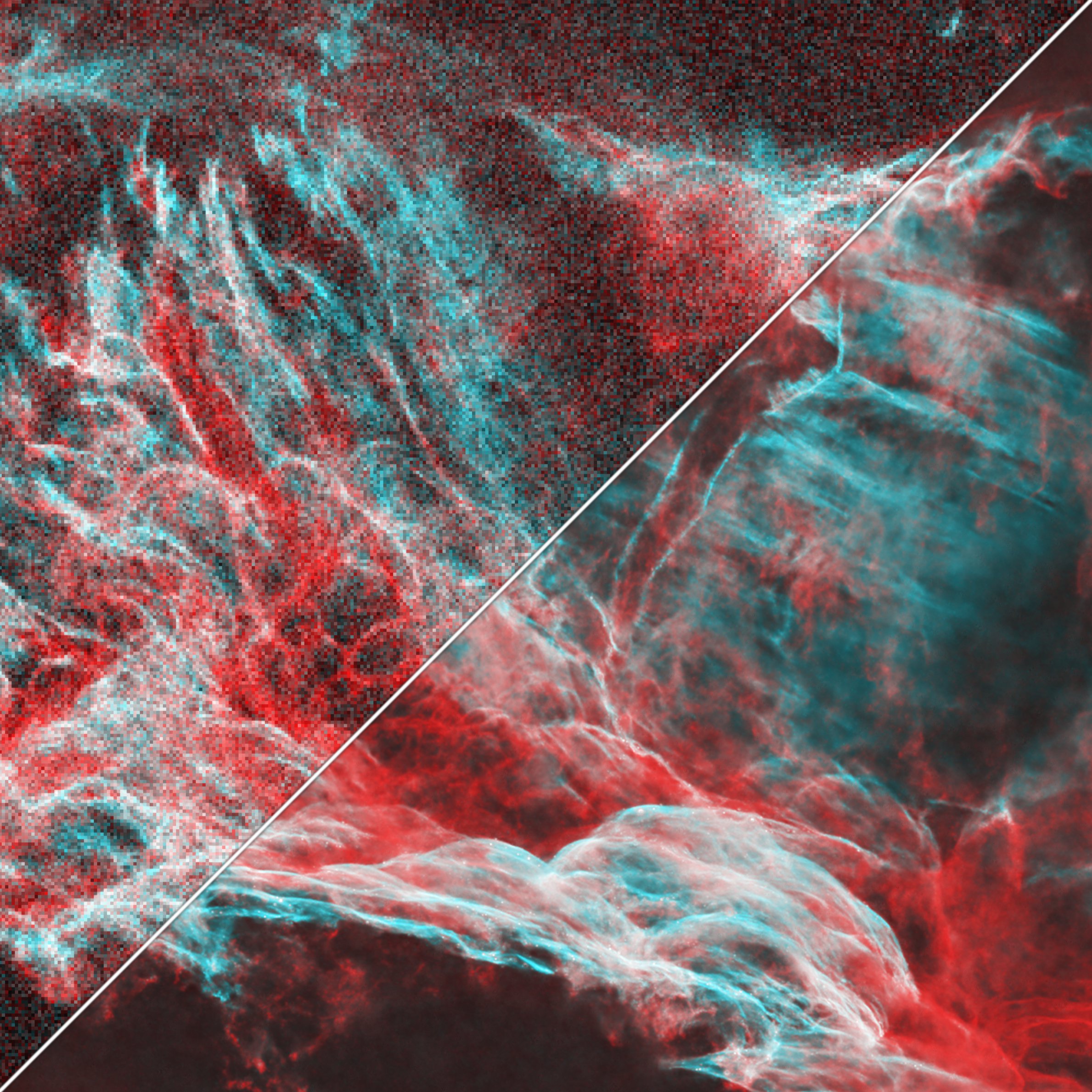
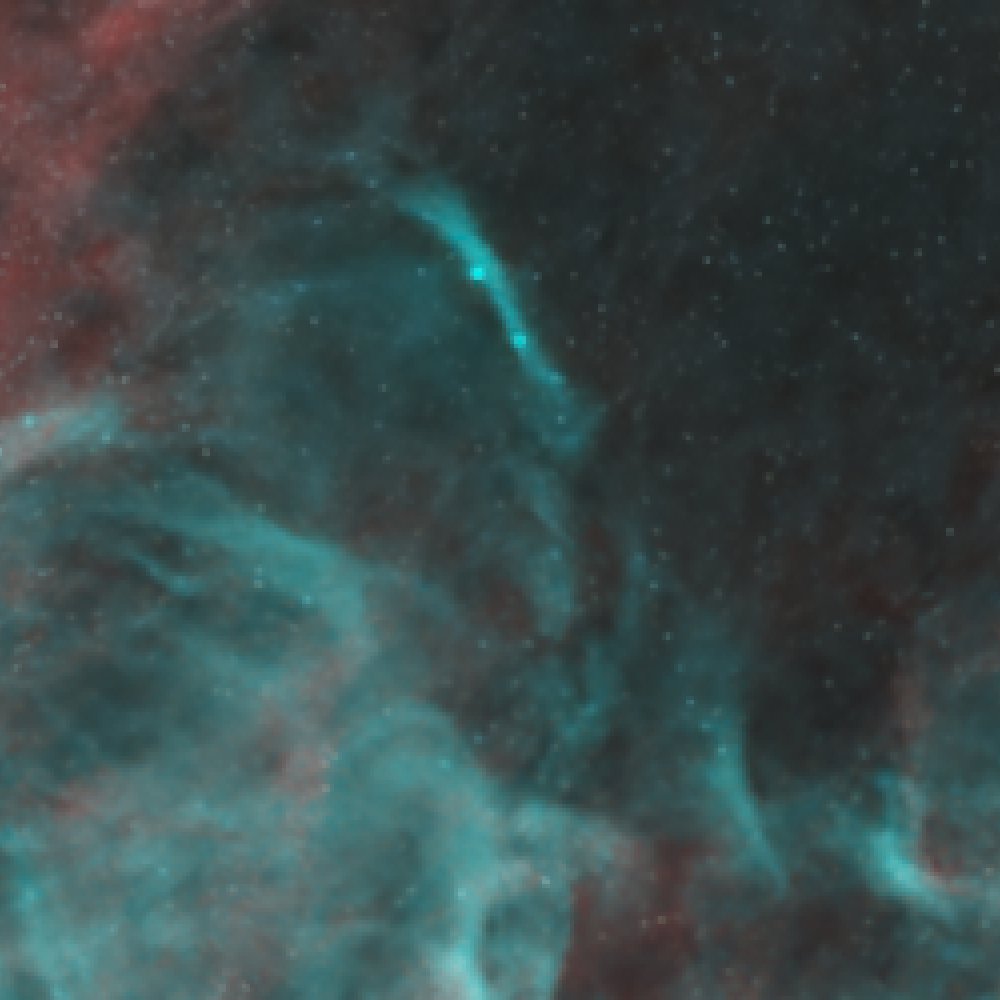
Before and after single channel DeepSNR
The Problem
While it may be tempting to perform certain processes to fake having a color image for DeepSNR to run, there are caveats and downsides to most of the trivial approaches one might think of.
Why Can’t I Convert the Image to Color?
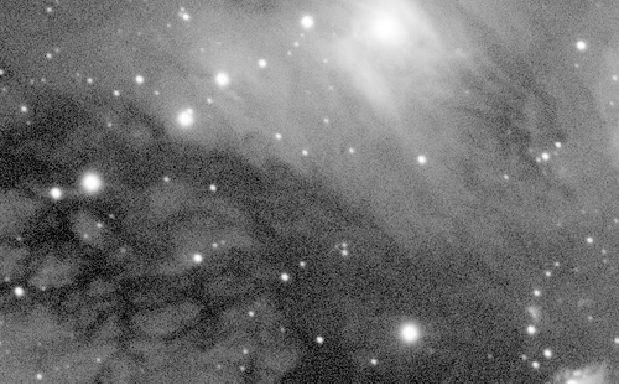
Performing DeepSNR on an HOO image hallucinates stars, creating distinct pockmark-like artifacts
As a result of DeepSNR being trained on color images only, it requires three channels that all contain distinct noise patterns. The technical term for this is ‘non-correlated’ noise, meaning no channel’s noise pattern depends on any of the others. It is able to use the difference in these noise patterns to get a “best guess” as to what the underlying signal might have been. When you convert a grayscale image to RGB, you only have one set of noise across all three channels, meaning it is strongly correlated, which will result in hallucinations.
Why Can’t I Add Noise?
While adding synthetic noise to an image to denoise it will allow DeepSNR to run with few hallucinations, adding noise will degrade the quality of the image post-denoise significantly. While the result may appear to work on the surface, adding more noise to the data causes the model to have to ‘guess’ more as to the true nature of the structure. If some part of the data were only on the edge of detectability before, adding more noise will destroy that signal. To retain the integrity of the data, we must explore other options.
When is it necessary?
It is important to note that it is only necessary to perform these techniques when you do not have appropriate data for DeepSNR’s normal operating conditions. For example, with RGB data alone, this is not necessary as you can just denoise an RGB combined image. However, there are several common cases where additional steps are necessary:
Captured Less than Three Channels
In any case where you capture less than three channels total, you will need to use one of the techniques outlined below. This is because DeepSNR strictly requires three non-correlated noise profiles, otherwise it will hallucinate stars and create obvious artifacts.
Channels do not Share Similar Structure
DeepSNR relies on all the channels sharing some amount of structure. If you combined three images with completely different structure and ran it through DeepSNR, you would notice ‘bleeding’ between the channels. This means that even if you have three channels of data, you may still want to denoise them individually. For example, supernova remnants will oftentimes have wildly different structures between Sii, Ha, and Oiii - this would be a good candidate for single channel noise reduction whereas a target like The Rosette nebula, may not be, as many of the structures are similar between the SHO channels.
Capturing LRGB Images
LRGB data presents another special edge case - oftentimes it is not necessary to treat luminance like a single channel as it can be combined with two of the other color channels to form a color image which can itself be denoised. eg. creating an RLB image (Where Lum is assigned to the Green channel), denoising that image, and then extracting the Green channel as the denoised Luminance.
Solutions
The two solutions both involve manipulating the available data in such a way as to form RGB images with non-correlated noise profiles. This requires some forethought as this can only be done in the pre-processing stages. As such, the two methods only diverge in the RGB image creation stage. The process is identical from that point on.
Method 1 — Drizzle Hack
The drizzle approach takes the least amount of effort and can be mostly automated. We will leverage the fact that drizzle can increase the pixel resolution of an image while retaining non-correlated noise profile to our advantage by abusing the Debayer process. The procedure is as follows:
- Drizzle Integration
For each channel, drizzle using a scale factor of at least 2 times. The resolution of the stack should be 2 times the final expected resolution.- Low drop shrink values create the least correlation between the noise and should be used, even if artifacts are created. Most drizzle artifacts will become invisible once downsampled in later steps.
- Debayer
On the drizzled master images, run the Debayer process with pattern set toRGGB, and the method set toSuperPixel. This will create an RGB image with half the pixel resolution of the grayscale image.- Superpixel debayering is effectively a 2x integer downsample that extracts color information. With RGGB, the top left pixel will be assigned to red, the top right and bottom left to green, and the bottom right to blue, forming one ‘SuperPixel’ with color data. Because the noise in the drizzled data was non-correlated, so too are the channels of color in the new RGB image.
That’s it! Now it’s time to move to the Processing RGB section to complete the process.
Method 2 — Triple Integration
In situations where the drizzle approach is not possible due to limitations of the data or in cases where there are too many subframes to drizzle in a reasonable amount of time, the triple integration method works just as well, but takes a bit more work. We will form three stacks from subsets of the original raw data and form those into a color image to be run through DeepSNR.
- Preparing the Data
For each channel, divide the calibrated and registered subframes into three roughly even groups. It is easiest to do this with three folders in the registered file directory.- For example, if I had 119 Hydrogen-alpha images, I would put 40 images in a folder called “Integration 1”, 40 into “Integration 2”, and 39 into “Integration 3”.
- Integrate
For each of the folders, integrate the images as your normally would, remembering to enable all appropriate subframe weighting and rejection parameters. - Combine RGB
You now have three mono integrations composed from equal subsets of the original data. Using Pixelmath or ChannelCombination, assign integrations 1, 2, 3 to RGB respectively to form a color image.
You may now proceed to the Processing RGB section!
Processing RGB
With the RGB color image created, we will finish up by performing the denoise and getting back a grayscale image.
- DeepSNR
On the new RGB image, apply DeepSNR at 100% with theLinear dataoption checked. The image will appear over-denoised, but this will be addressed in step three.- Alternatively, you can apply DeepSNR at your desired strength now, however it may be hard to judge exactly what strength is right for the data and running many iterations can become lengthy.
- If when the STF is applied and you see a dominant hue, change the stretch preview to ‘unlinked’ by ctrl-clicking the nuclear button in the top right, or disabling the chain link icon in the STF process. The unlinked stretch should look approximately neutral in color.
- PixelMath
Again to the RGB image, apply the following PixelMath withCreate new Imagechecked,Color spaceset to Grayscale, and the identifier set toNR. This averages the three color channels, creating a single gray output./*file: "RGB/k"*/Avg($T[0],$T[1],$T[2]) - Blending
In step one, DeepSNR was set to 100%, we will blend this back with the original to create a natural noise profile. If you used the drizzle method, apply an IntegerResample set to 2x downsample and name this imageOrg. If you used the Triple Integration method, bring in the stack containing all data and name itOrg. Then in PixelMath, use the following expression to quickly iterate denoise amounts./*file: "RGB/k"*/(Org * F) + (NR * ~F)/*file: "Symbols"*/F = 0.7- Adjust the value of
Fon the range of 0 to 1 inSymbolsto achieve a pleasing noise profile.
- Adjust the value of
Please feel free to contact me with any questions!
See my Contact page for info on how to contact me!